New research shows us the role of uncertainty in depth conversion, and it can be more relevant than you think.

It’s not precisely today’s news. Given the sparse data we have to produce a model several kilometers below the surface, it comes as a given that what we get is different from what is there. Consider the enormity of the entire process. Seismic acquisition is performed with more or less accuracy depending on location and investment made. This data is processed through a series of algorithms such as filtering, stacking, or migration. A geophysicist, often subjectively, interprets the data in its natural time unit. And then, using one of the multiple possible approaches, depth converts that interpretation to a, hopefully, coherent and structurally reasonable depth model. And now the question arises: where should we drill and how much of the resource can we expect?

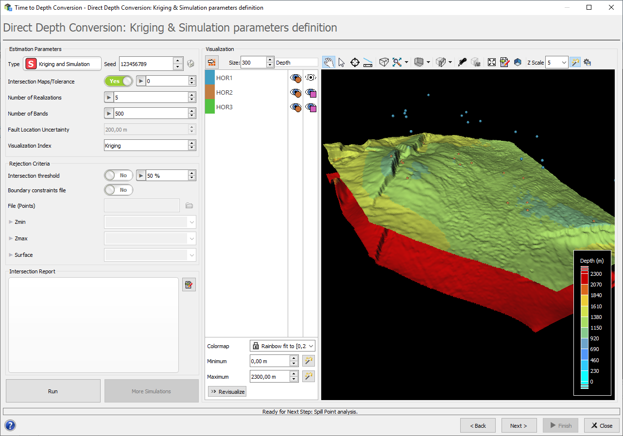
Invariably the answer is complex. Recently we have developed a new tool in depth conversion (Isatis.neo – Petroleum edition) that allows the use of multiple conversion methodologies, and the introduction of different sources of uncertainty (explored with stochastic simulation). Having it all together in the same package made experimentation an easier endeavor. And the results are discouraging for one used to always follow the same methodology. When calculating the volumes over the results of different conversion scenarios, such as purely sequential conversion, joint conversion, or anything in between, we have obtained differences up to the order of magnitude for the same layer. Furthermore, when adding other sources of uncertainty such as interpretation uncertainty, or fault position uncertainty, some of the realizations returned different structural scenarios. All of this is potentially useful information, but a common concern about dealing with multiple realizations of the same entity is what to do with that information. Even if this uncertainty is acknowledged, we can’t move forward in the process of reservoir characterization with what seems an excessive amount of data. But that would be missing the point.

So how do we manage the uncertainty space of our case study? By reducing it to meaningful categories. Let’s take an example of another recent research. Using a case study of a top reservoir horizon cut by a major fault, we knew intuitively where the main trap should be. Yet at least one other structure close by seemed to be ideal for a smaller trap. By converting this case study and considering fault uncertainty, we’ve obtained a set of realizations. In about a third of those realizations, these two traps were merged into one. The question now was not what to do with dozens or hundreds of simulations. It was about how to prove or disprove the meaningfully different scenarios we obtained in a very significant percentage of our realizations. A far more pragmatic question to answer that has far-reaching implications for all the operations that follow.

So, do not look at a set of realizations as something that just produces probability curves instead of single definite values. Careful observation of that uncertainty data can often be reduced to two or three relevant scenarios. And by confirming or refuting those hypotheses, you are effectively increasing the accuracy of your model. It is the main reason that leads us to the creation of our Time to Depth conversion workflow. An open platform that allows free and easy experimentation and analysis in depth conversion technologies. A tool that gives the user the means to explore all credible scenarios.